


A Numerical Method for Solving Three-Dimensional Probability Distribution of Rockmass Fracture Orientations
-
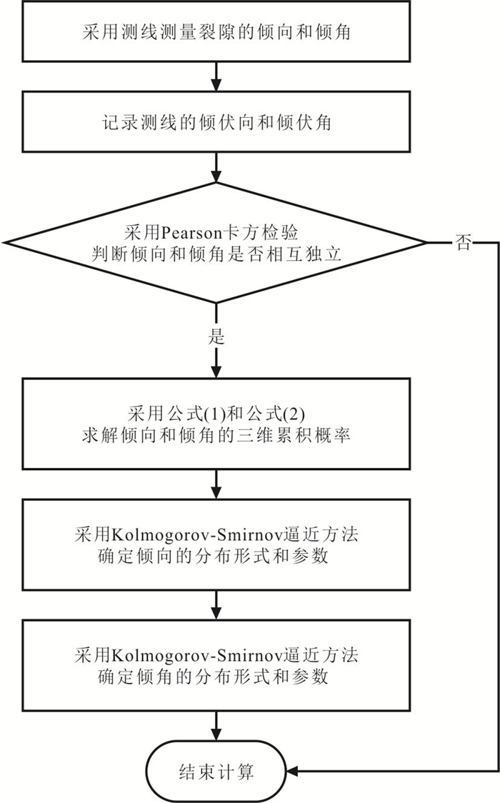
摘要: 测线法是一种广泛使用的裂隙几何特征野外观测技术,但它获得的一维产状观测数据不能代表三维空间内的概率分布.在实测裂隙倾向和倾角之间相互独立的假设基础上,借用概率论和微积分建立了一维数据和三维分布的数值解关系式,进而提出一种由一维观测数据求解三维概率分布的方法.该方法的实现步骤是:(1)通过关系式数值求解产状的三维累积概率;(2)使用如Kolmogorov-Smirnov逼近法对累积概率进行分布形式和分布参数的估计.结合两类裂隙(层理面和节理面)的观测数据,比较了本文方法与Fouché方法的求解误差,并调查了样本容量对本文方法求解误差的影响.结果表明,本文方法求解误差更低.样本容量接近150时,可实现最低求解误差;当超过150时,求解误差不会随样本容量的增加而显著降低.同时,应用于互不平行的裂隙个体如节理面时,本文方法效果明显.而应用于近似平行的裂隙个体如层理面时,效果不明显.Abstract: The scanline mapping is a widely-used 1D field technique for fracture geometry observation. However, the 1D orientation observations from this technique poorly represent the 3D probability distribution. In this work, a numerical method for solving the 3D probability distribution of orientations is presented. It makes the assumption of observed dip direction-angle independence and adopts a mathematical relationship between the 1D observations and the 3D distribution. This method follows a two-step procedure that first using the relationship to solve the 3D cumulative, and then estimating the distribution type and parameters over the probabilities by employing the Kolmogorov-Smirnov approximation. Two cases of fractures (bedding planes and joints) illustrate that the presented method provides a smaller-error solution in comparison with the Fouché method. The minimum solution error of the presented method can be attained when the sample size is closely 150; if the sample size exceeds this value, the solution error will not decrease significantly as sample size increases. Moreover, the effectiveness of the presented method is investigated. The results show that the presented method performs effectively when applied to non-parallel fracture individuals, e.g. joints, whereas with low effectiveness when applied to sub-parallel fracture individuals, e.g. bedding planes.
-
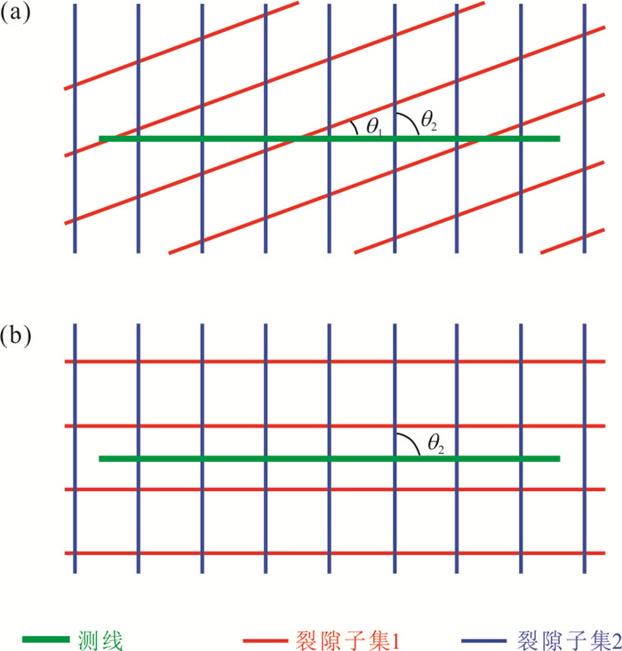
图 1 测线与裂隙交切关系模型(二维概化)
假设包含于同一裂隙组的两个子集,子集1和子集2.图a为测线与子集1的夹角小于测线与子集2的夹角,即θ1 < θ2;图b为极端情况θ1=0° < θ2
Fig. 1. Illustration of intersection of scanline to fractures
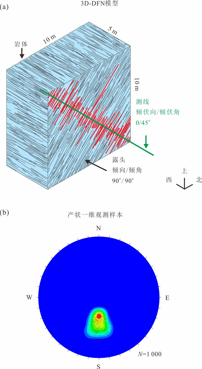
图 3 3D-DFN模型和其上的产状一维观测样本
a. 3D-DFN模型,红线表示测线技术观测的裂隙;b.产状一维观测样本,采用上半球等角度赤平投影成图,N代表样本容量
Fig. 3. 3D-DFN model and 1D orientation sample
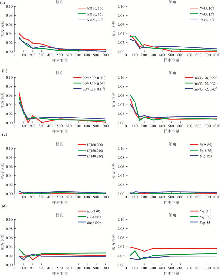
图 4 根方误差-样本容量
a.三维产状服从正态分布,左图为倾向,右图为倾角;b. 对数正态分布;c.均匀分布;d.指数分布
Fig. 4. Root square error versus sample size
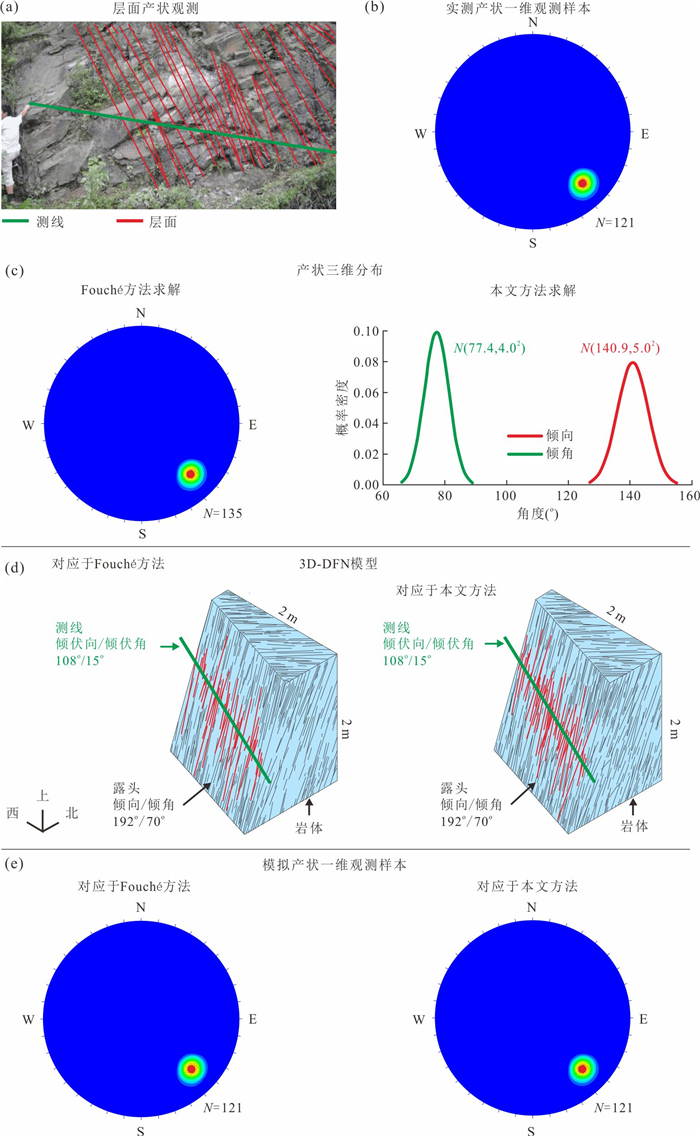
图 5 案例Ⅰ
a.采用测线观测层理面产状;b.实测产状一维观测样本;c.产状三维分布,左图是Fouché方法求解的,右图是本文方法求解的;d. 3D-DFN模型,红线表示被测线技术观测的裂隙,左图建模参数是Fouché方法求解的产状三维分布,右图建模参数是本文方法求解的产状三维分布;e.模拟产状一维观测样本,左图取样于Fouché方法求解的产状三维分布构建的模型,右图取样于本文方法求解的产状三维分布构建的模型
Fig. 5. Case Ⅰ
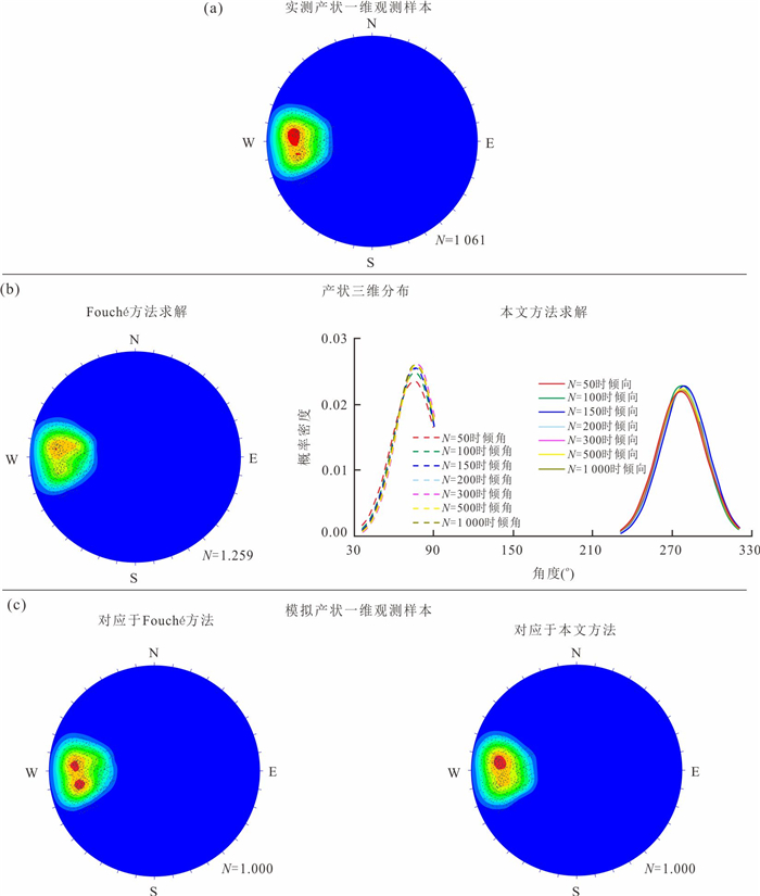
图 6 案例Ⅱ
a.实测产状一维观测样本;b.产状三维分布,左图是Fouché方法求解的,右图是本文方法求解的;c. 模拟产状一维观测样本,左图取样于Fouché方法求解的产状三维分布构建的模型,右图取样于本文方法求解的产状三维分布构建的模型
Fig. 6. Case Ⅱ
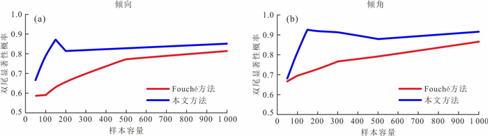
图 7 双尾显著性概率-样本容量
双尾显著性概率定量表达了模拟样本与实测样本在分布上的差异大小.a.倾向;b.倾角
Fig. 7. Two-tailed significance versus sample size
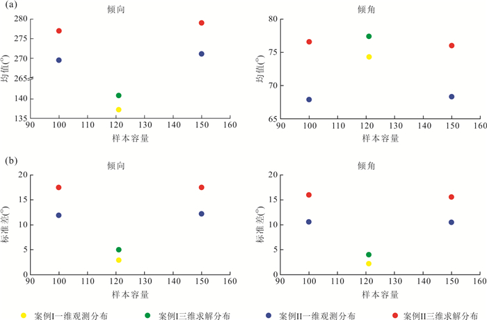
图 8 一维产状观测分布和本文方法求解的三维分布的参数对比
a.均值,左图是倾向,右图是倾角;b.标准差
Fig. 8. Comparison of 1D observation distribution parameters and 3D distribution parameters solved using the proposed method
表 1 3D-DFN建模参数
Table 1. 3D-DFN modeling parameters
体密度(m-3) 模拟区 应用区 测线 长(m) 宽(m) 高(m) 长(m) 宽(m) 高(m) 倾伏向(°) 倾伏角(°) 7 30 30 30 20 20 20 0 45 模型 产状 半径(m) 样本容量 倾向(°) 倾角(°) Ⅰ N(180, 102) N(45, 102) Exp(1.5) 50/100/150/200/300/500/1 000 Ⅱ N(180, 152) N(45, 152) Exp(1.5) 50/100/150/200/300/500/1 000 Ⅲ N(180, 202) N(45, 202) Exp(1.5) 50/100/150/200/300/500/1 000 Ⅳ lnN(5.19, 0.062) lnN(3.78, 0.222) Exp(1.5) 50/100/150/200/300/500/1 000 Ⅴ lnN(5.19, 0.082) lnN(3.75, 0.322) Exp(1.5) 50/100/150/200/300/500/1 000 Ⅵ lnN(5.19, 0.112) lnN(3.72, 0.422) Exp(1.5) 50/100/150/200/300/500/1 000 Ⅶ U(160, 200) U(25, 65) Exp(1.5) 50/100/150/200/300/500/1 000 Ⅷ U(150, 210) U(15, 75) Exp(1.5) 50/100/150/200/300/500/1 000 Ⅸ U(140, 220) U(5, 85) Exp(1.5) 50/100/150/200/300/500/1 000 Ⅹ Exp(180) Exp(45) Exp(2.5) 50/100/150/200/300/500/1 000 Ⅺ Exp(185) Exp(50) Exp(2.5) 50/100/150/200/300/500/1 000 Ⅻ Exp(190) Exp(55) Exp(2.5) 50/100/150/200/300/500/1 000 注:表中N(i,j2)为正态分布,其中i表示均值,j表示标准差;Exp(k)为指数分布,其中k表示均值;lnN(l,m2)为对数正态分布,其中l表示位置参数,m表示比例参数;U(n,p)为均匀分布,其中n表示上限,p表示下限.  下载: 导出CSV
表 2 采用Pearson卡方检验获得的产状独立性测试结果
Table 2. Orientation independence output using the Pearson chi-square test
样本M-s 显著性概率 样本M-s 显著性概率 样本M-s 显著性概率 样本M-s 显著性概率 样本M-s 显著性概率 样本M-s 显著性概率 Ⅰ-50 0.528 Ⅲ-50 0.819 Ⅴ-50 0.492 Ⅶ-50 0.512 Ⅸ-50 0.452 Ⅺ-50 0.429 Ⅰ-100 0.526 Ⅲ-100 0.330 Ⅴ-100 0.827 Ⅶ-100 0.987 Ⅸ-100 0.475 Ⅺ-100 0.863 Ⅰ-150 0.497 Ⅲ-150 0.592 Ⅴ-150 0.874 Ⅶ-150 0.835 Ⅸ-150 0.778 Ⅺ-150 0.537 Ⅰ-200 0.259 Ⅲ-200 0.460 Ⅴ-200 0.629 Ⅶ-200 0.926 Ⅸ-200 0.565 Ⅺ-200 0.292 Ⅰ-300 0.636 Ⅲ-300 0.673 Ⅴ-300 0.810 Ⅶ-300 0.562 Ⅸ-300 0.472 Ⅺ-300 0.415 Ⅰ-500 0.773 Ⅲ-500 0.550 Ⅴ-500 0.754 Ⅶ-500 0.789 Ⅸ-500 0.969 Ⅺ-500 0.217 Ⅰ-1000 0.830 Ⅲ-1000 0.543 Ⅴ-1000 0.424 Ⅶ-1000 0.733 Ⅸ-1000 0.987 Ⅺ-1000 0.246 Ⅱ-50 0.297 Ⅳ-50 0.756 Ⅵ-50 0.396 Ⅷ-50 0.954 X-50 0.992 Ⅻ-50 0.942 Ⅱ-100 0.327 Ⅳ-100 0.344 Ⅵ-100 0.607 Ⅷ-100 0.486 X-100 0.907 Ⅻ-100 0.859 Ⅱ-150 0.316 Ⅳ-150 0.483 Ⅵ-150 0.256 Ⅷ-150 0.518 X-150 0.704 Ⅻ-150 0.803 Ⅱ-200 0.252 Ⅳ-200 0.301 Ⅵ-200 0.316 Ⅷ-200 0.487 X-200 0.874 Ⅻ-200 0.925 Ⅱ-300 0.593 Ⅳ-300 0.912 Ⅵ-300 0.313 Ⅷ-300 0.981 X-300 0.838 Ⅻ-300 0.478 Ⅱ-500 0.505 Ⅳ-500 0.568 Ⅵ-500 0.372 Ⅷ-500 0.702 X-500 0.483 Ⅻ-500 0.938 Ⅱ-1000 0.524 Ⅳ-1000 0.089 Ⅵ-1000 0.552 Ⅷ-1000 0.433 X-1000 0.209 Ⅻ-1000 0.260 注:样本M-s中M是模型编号、s是样本容量.显著性概率指的是双尾值.
下载: 导出CSV
表 3 本文方法求解的产状三维概率分布
Table 3. 3D probability distribution of orientations solved using the presented method
样本 产状 样本 产状 倾向(°) 倾角(°) 倾向(°) 倾角(°) Ⅰ-50 N(178.3, 8.02) N(46.1, 8.12) Ⅶ-50 U(160.3, 200.2) U(25.0, 64.9) Ⅰ-100 N(178.8, 8.52) N(46.5, 8.92) Ⅶ-100 U(160.4, 199.9) U(25.0, 64.9) Ⅰ-150 N(179.3, 8.52) N(45.6, 9.42) Ⅶ-150 U(160.3, 199.9) U(25.0, 64.9) Ⅰ-200 N(179.0, 9.22) N(45.3, 9.02) Ⅶ-200 U(160.3, 199.9) U(25.0, 64.9) Ⅰ-300 N(178.9, 9.42) N(45.5, 9.42) Ⅶ-300 U(160.1, 199.9) U(25.0, 65.0) Ⅰ-500 N(179.5, 10.12) N(45.0, 10.12) Ⅶ-500 U(160.1, 200.1) U(25.0, 65.0) Ⅰ-1000 N(179.7, 10.22) N(45.0, 10.12) Ⅶ-1000 U(160.0, 200.1) U(25.0, 65.0) Ⅱ-50 N(176.9, 13.72) N(46.2, 11.62) Ⅷ-50 U(154.5, 217.6) U(13.0, 72.1) Ⅱ-100 N(177.6, 14.92) N(45.9, 11.52) Ⅷ-100 U(153.5, 212.9) U(11.4, 71.7) Ⅱ-150 N(178.2, 15.12) N(45.8, 12.72) Ⅷ-150 U(151.7, 211.8) U(12.9, 72.0) Ⅱ-200 N(178.6, 15.32) N(45.2, 13.92) Ⅷ-200 U(152.2, 211.4) U(12.5, 71.2) Ⅱ-300 N(178.9, 15.32) N(44.8, 14.12) Ⅷ-300 U(150.7, 209.9) U(13.6, 73.2) Ⅱ-500 N(178.8, 14.72) N(45.2, 14.32) Ⅷ-500 U(150.8, 209.5) U(14.2, 74.1) Ⅱ-1000 N(179.4, 15.32) N(45.4, 14.72) Ⅷ-1000 U(150.3, 210.2) U(15.2, 73.7) Ⅲ-50 N(185.2, 16.62) N(43.5, 15.72) Ⅸ-50 U(145.9, 215.2) U(2.0, 82.0) Ⅲ-100 N(184.4, 18.92) N(40.2, 18.22) Ⅸ-100 U(141.3, 218.9) U(1.4, 78.5) Ⅲ-150 N(184.0, 19.92) N(43.2, 19.82) Ⅸ-150 U(142.4, 219.5) U(2.7, 80.4) Ⅲ-200 N(182.5, 19.22) N(43.2, 18.92) Ⅸ-200 U(142.4, 213.6) U(3.0, 80.6) Ⅲ-300 N(181.9, 18.62) N(44.5, 18.02) Ⅸ-300 U(141.3, 219.0) U(3.8, 81.6) Ⅲ-500 N(180.9, 18.92) N(43.1, 18.42) Ⅸ-500 U(142.8, 214.0) U(5.7, 82.7) Ⅲ-1000 N(180.2, 19.82) N(44.5, 18.92) Ⅸ-1000 U(140.1, 218.8) U(6.2, 84.1) Ⅳ-50 lnN(5.203, 0.0382) lnN(3.819, 0.1662) X-50 Exp(355.5) Exp(87.4) Ⅳ-100 lnN(5.198, 0.0502) lnN(3.803, 0.1972) X-100 Exp(311.6) Exp(83.1) Ⅳ-150 lnN(5.200, 0.0552) lnN(3.795, 0.2222) X-150 Exp(107.3) Exp(79.1) Ⅳ-200 lnN(5.199, 0.0562) lnN(3.797, 0.2082) X-200 Exp(133.1) Exp(72.6) Ⅳ-300 lnN(5.198, 0.0552) lnN(3.796, 0.2112) X-300 Exp(102.6) Exp(82.5) Ⅳ-500 lnN(5.196, 0.0572) lnN(3.796, 0.2202) X-500 Exp(104.5) Exp(81.7) Ⅳ-1000 lnN(5.194, 0.0562) lnN(3.796, 0.2162) X-1000 Exp(109.0) Exp(82.2) Ⅴ-50 lnN(5.210, 0.0552) lnN(3.869, 0.2422) Ⅺ-50 Exp(81.7) Exp(71.7) Ⅴ-100 lnN(5.199, 0.0702) lnN(3.831, 0.2562) Ⅺ-100 Exp(104.6) Exp(85.8) Ⅴ-150 lnN(5.194, 0.0772) lnN(3.752, 0.3102) Ⅺ-150 Exp(118.4) Exp(62.9) Ⅴ-200 lnN(5.199, 0.0752) lnN(3.764, 0.2952) Ⅺ-200 Exp(110.9) Exp(61.9) Ⅴ-300 lnN(5.197, 0.0772) lnN(3.752, 0.3062) Ⅺ-300 Exp(102.5) Exp(70.6) Ⅴ-500 lnN(5.194, 0.0772) lnN(3.757, 0.2962) Ⅺ-500 Exp(99.9) Exp(73.2) Ⅴ-1000 lnN(5.194, 0.0782) lnN(3.755, 0.3022) Ⅺ-1000 Exp(99.1) Exp(76.5) Ⅵ-50 lnN(5.210, 0.0762) lnN(3.845, 0.3492) Ⅻ-50 Exp(116.3) Exp(69.5) Ⅵ-100 lnN(5.197, 0.0882) lnN(3.801, 0.3762) Ⅻ-100 Exp(141.4) Exp(68.1) Ⅵ-150 lnN(5.196, 0.1032) lnN(3.757, 0.3942) Ⅻ-150 Exp(114.6) Exp(66.7) Ⅵ-200 lnN(5.192, 0.1012) lnN(3.768, 0.3882) Ⅻ-200 Exp(107.0) Exp(72.9) Ⅵ-300 lnN(5.192, 0.0992) lnN(3.755, 0.3982) Ⅻ-300 Exp(117.6) Exp(71.7) Ⅵ-500 lnN(5.193, 0.0982) lnN(3.759, 0.3932) Ⅻ-500 Exp(117.9) Exp(76.9) Ⅵ-1000 lnN(5.191, 0.1022) lnN(3.763, 0.3912) Ⅻ-1000 Exp(118.7) Exp(77.4)
下载: 导出CSV
表 4 3D-DFN建模部分参数
Table 4. 3D-DFN modeling partial parameters
体密度(m-3) 直径(m) 隙宽(mm) 模拟区 长(m) 宽(m) 高(m) 4 Exp(0.5) Exp(1.2) 10 10 10
下载: 导出CSV
-
Alghalandis, Y.F., 2017. ADFNE: Open Source Software for Discrete Fracture Network Engineering, Two and Three Dimensional Applications. Computers & Geosciences, 102: 1-11. https://doi.org/10.1016/j.cageo.2017.02.002 Berrone, S., Canuto, C., Pieraccini, S., et al., 2015. Uncertainty Quantification in Discrete Fracture Network Models: Stochastic Fracture Transmissivity. Computers & Mathematics with Applications, 70(4): 603-623. https://doi.org/10.1016/j.camwa.2015.05.013 Bisdom, K., Bertotti, G., Bezerra, F.H., 2017. Inter-Well Scale Natural Fracture Geometry and Permeability Variations in Low-Deformation Carbonate Rocks. Journal of Structural Geology, 97: 23-36. https://doi.org/10.1016/j.jsg.2017.02.011 Brereton, R.G., 2015. The Chi Squared and Multinormal Distributions. Journal of Chemometrics, 29(1): 9-12. https://doi.org/10.1002/cem.2680 Carvalho, L., 2015. An Improved Evaluation of Kolmogorov's Distribution. Journal of Statistical Software, 65(3): 1-7. https://doi.org/10.18637/jss.v065.c03 Follin, S., Hartley, L., Rhén, I., et al., 2014. A Methodology to Constrain the Parameters of a Hydrogeological Discrete Fracture Network Model for Sparsely Fractured Crystalline Rock, Exemplified by Data from the Proposed High-Level Nuclear Waste Repository Site at Forsmark, Sweden. Hydrogeology Journal, 22(2): 313-331. https://doi.org/10.1007/s10040-013-1080-2 Fouché, O., Diebolt, J., 2004. Describing the Geometry of 3D Fracture Systems by Correcting for Linear Sampling Bias. Mathematical Geology, 36(1): 33-63. https://doi.org/10.1023/B:MATG.0000016229.37309.fd Kang, J.T., Wu, Q., Tang, H.M., et al., 2019. Strength Degradation Mechanism of Soft and Hard Interbedded Rock Masses of Badong Formation Caused by Rock/Discontinuity Degradation. Earth Science, 44(11): 3950-3960(in Chinese with English abstract). Kolmogorov, A.N., 1933. Foundations of Probability. American Mathematical Society Chelsea Publishing Company, Houston, Texas. Manda, A.K., Mabee, S.B., 2010. Comparison of Three Fracture Sampling Methods for Layered Rocks. International Journal of Rock Mechanics and Mining Sciences, 47(2): 218-226. https://doi.org/10.1016/j.ijrmms.2009.12.004 Mauldon, M., Mauldon, J.G., 1997. Fracture Sampling on a Cylinder: From Scanlines to Boreholes and Tunnels. Rock Mechanics and Rock Engineering, 30(3): 129-144. https://doi.org/10.1007/BF01047389 Peacock, D.C.P., Harris, S.D., Mauldon, M., 2003. Use of Curved Scanlines and Boreholes to Predict Fracture Frequencies. Journal of Structural Geology, 25(1): 109-119. https://doi.org/10.1016/S0191-8141(02)00016-0 Pearson, K.X., 1900. On the Criterion That a Given System of Deviations from the Probable in the Case of a Correlated System of Variables is Such That It can be Reasonably Supposed to have Arisen from Random Sampling. The London, Edinburgh, and Dublin Philosophical Magazine and Journal of Science, 50 (302): 157-175. doi: 10.1080/14786440009463897 Roy, P., du Frane, W.L., Kanarska, Y., et al., 2016. Numerical and Experimental Studies of Particle Settling in Real Fracture Geometries. Rock Mechanics and Rock Engineering, 49(11): 4557-4569. https://doi.org/10.1007/s00603-016-1100-3 Ruan, Y.K., Chen, J.P., Li, Y.Y., et al., 2016. Identification of Homogeneous Structural Domains of Jointed Rock Masses Based on Joint Occurrence and Trace Length. Rock and Soil Mechanics, 37(7): 2028-2032(in Chinese with English abstract). Smirnov, N., 1948. Table for Estimating the Goodness of Fit of Empirical Distributions. The Annals of Mathematical Statistics, 19(2): 279-281. doi: 10.1214/aoms/1177730256 Tang, H.M., Huang, L., Bobet, A., et al., 2016. Identification and Mitigation of Error in the Terzaghi Bias Correction for Inhomogeneous Material Discontinuities. Strength of Materials, 48(6): 825-833. https://doi.org/10.1007/s11223-017-9829-9 Tang, H.M., Huang, L., Juang, C.H., et al., 2017. Optimizing the Terzaghi Estimator of the 3D Distribution of Rock Fracture Orientations. Rock Mechanics and Rock Engineering, 50(8): 2085-2099. https://doi.org/10.1007/s00603-017-1254-7 Tang, H.M., Zhang, J.R., Huang, L., et al., 2018. Correction of Line-Sampling Bias of Rock Discontinuity Orientations Using a Modified Terzaghi Method. Advances in Civil Engineering, 2018: 1-9. https://doi.org/10.1155/2018/1629039 Terzaghi, R.D., 1965. Sources of Error in Joint Surveys. Géotechnique, 15(3): 287-304. https://doi.org/10.1680/geot.1965.15.3.287 Williams-Stroud, S., Ozgen, C., Billingsley, R.L., 2013. Microseismicity-Constrained Discrete Fracture Network Models for Stimulated Reservoir Simulation. Geophysics, 78(1): B37-B47. https://doi.org/10.1190/geo2011-0061.1 Xia, D., Ge, Y.F., Tang, H.M., et al., 2020. Segmentation of Region of Interest and Identification of Rock Discontinuities in Digital Borehole Images. Earth Science, 45(11): 4207-4217(in Chinese with English abstract). Zaree, V., Riahi, M.A., Khoshbakht, F., et al., 2016. Estimating Fracture Intensity in Hydrocarbon Reservoir: An Approach Using DSI Data Analysis. Carbonates and Evaporites, 31(1): 101-107. https://doi.org/10.1007/s13146-015-0246-5 亢金涛, 吴琼, 唐辉明, 等, 2019. 岩石/结构面劣化导致巴东组软硬互层岩体强度劣化的作用机制. 地球科学, 44(11): 3950-3960. doi: 10.3799/dqkx.2019.110 阮云凯, 陈剑平, 李严严, 等, 2016. 基于裂隙产状和迹长划分岩体统计均质区研究. 岩土力学, 37(7): 2028-2032. https://www.cnki.com.cn/Article/CJFDTOTAL-YTLX201607025.htm 夏丁, 葛云峰, 唐辉明, 等, 2020. 数字钻孔图像兴趣区域分割与岩体结构面特征识别. 地球科学, 45(11): 4207-4217. doi: 10.3799/dqkx.2020.003 -
 赵萌 附件1.docx

-

 点击查看大图
计量
- 文章访问数: 1606
- HTML全文浏览量: 586
- PDF下载量: 95
- 被引次数: 0
